要約
This application note discusses how to get more accurate readings from ultrasonic transducers used in liquid and gas flow meters. It describes a software compensation technique used to overcome flow-rate readings that might be inaccurate because of characteristic differences between measurement devices.
Introduction
This application note describes a software compensation technique that reduces time-offset errors over temperature. Ultrasonic transducers used for flow measurement can have substantial characteristic differences from one device to the next. In applications that require high accuracy, such as liquid and gas flow meters, these differences can impart temperature-dependent offsets in the time-difference measurements that time-to-digital converters—such as the MAX3510x devices—return. This results in calculated flow rates that are often offset from the actual flow rate.
Zero-flow, constant temperature experiments with 500kHz gas transducers, for example, have registered time offsets (Δτ) of as much as 50ns; offset changes from 10°C to 40°C registered as high as 10ns.
Transducer Behavior Hypothesis
MAX3510x devices apply an excitation signal to the transmitting transducer. The signal is a square wave of programmable frequency and duration. The transducer responds to this signal by vibrating in a way that is not only dependent on the input frequency spectrum (predominately odd harmonics) but also on internal characteristics. The resulting acoustic waveform contains a frequency spectrum that is different from the source.
A similar situation exists with the receiving transducer. The received acoustic waveform and the electrical spectrum emitted by the receiving transducer are also different. The aggregate of these differences manifests itself in the time domain as a dynamic delay.
If both transducers have identical characteristics, then this delay error is the same in both directions. They would, therefore, cancel out during the delta-time calculation that is required to determine the flow rate. Transducers of the same model and manufacturing batch, however, have been found to have significantly different electromechanical characteristics. Moreover, the predominate transducer characteristics are sensitive to temperature. These deviations from ideal behavior require per-unit compensation for most flow-measuring applications.
Equation 1 expresses the problem mathematically, as follows:
Δτ = (τu + τu𝑒) - (τd + τd𝑒)
where,
Δτ = time difference measurement necessary for flow calculations, TOF_DIFF, from the MAX3510x
τu = actual time of flight in the Up direction
τd = actual time of flight in the Down direction
τu𝑒 = aggregate time error in the Up direction
τd𝑒 = aggregate time error in the Down direction
In perfectly matched transducers, τu𝑒 = τd𝑒, and therefore they fall out of the equation. In actual transducers, the second equation indicates it is expected that τu𝑒 - τd𝑒 can be approximated by a function of temperature specific to the transducer pair:
ƒ𝑒(τ) = τu𝑒 - τd𝑒
Combining the first and second equation, then, we have Equation 3, as follows:
Δτ = ƒ𝑒(τ) + τu - τd
Therefore, to obtain actual time-of-flight difference, Δ'τ, we compensate Equation 3 with -ƒ𝑒(τ), as Equation 4 below shows:
Δ'τ = Δτ - ƒ𝑒(τ)
Approach
The phenomena represented by τu𝑒 and τd𝑒 are complex. Instead of attempting to develop a rigorous model, we use an experimental approach based on the hypothesis presented above.
Initial tests consisted of four test devices (no. 10, no. 11, no. 12, and no. 16). Each test device comprised a closed, air-filled tube with a 500kHz generic transducer at either end, driven by a MAX32625MBED board with a MAX35104EVKIT2 Arduino shield. The closed tube ensured that net material flow within the tube was practically zero. The temperature was maintained at approximately 10°C ± 0.5°C over a 7.5-hour period, and Δτ was recorded. Figure 1 shows the baseline results for the four test devices.
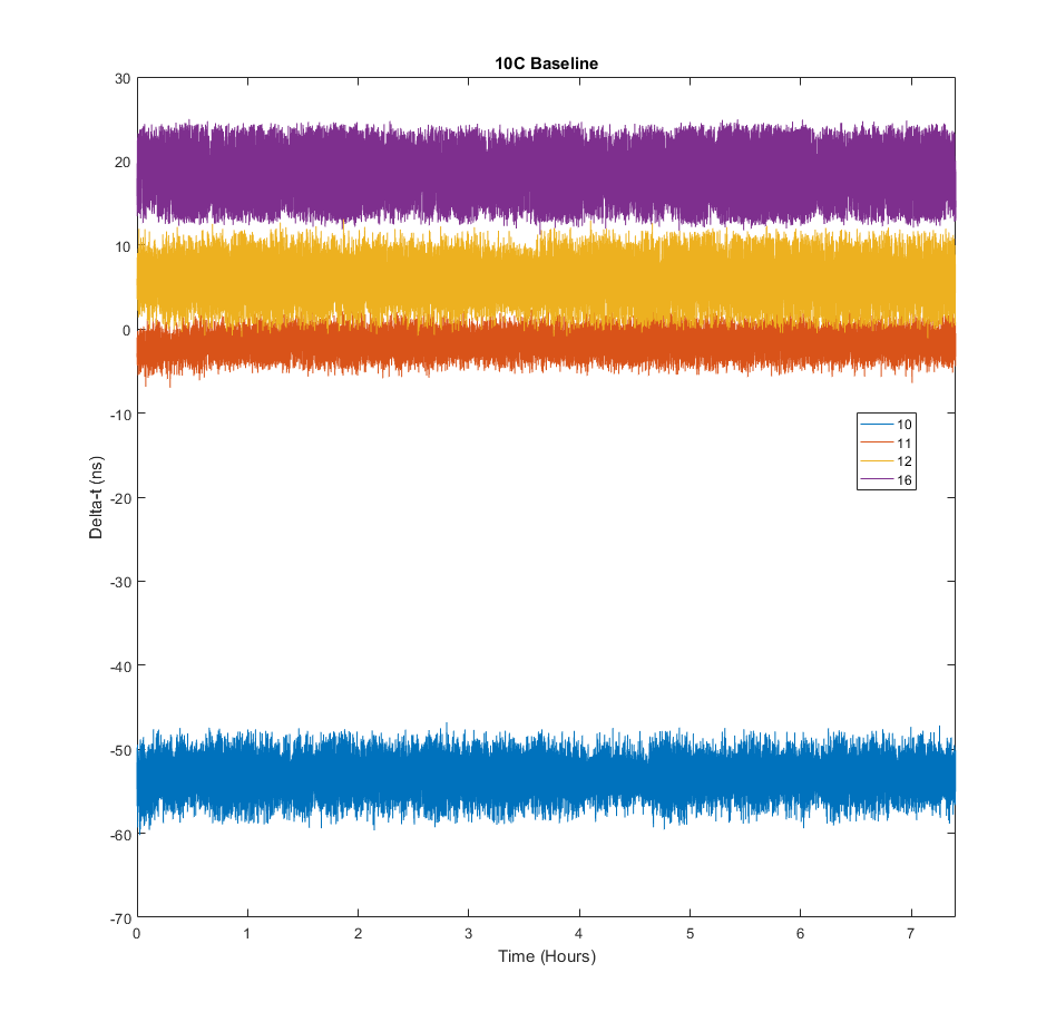
Figure 1. 10C baseline.
Table 1 shows that the results revealed that ƒ𝑒(τ) was constant with less than 3ns standard deviation, but significantly different for each unit under test. Further, when the polarity of the tube was reversed (the Up transducer swapped with the Down transducer in each tube), the sign of ƒ𝑒(τ) changed accordingly.
| DUT ID# | ƒ𝑒(10) | Standard Deviation (ns) |
| 10 | -53.2E-09 | 2.12E-09 |
| 11 | -1.63E-09 | 1.41E-09 |
| 12 | 5.83E-09 | 2.50E-09 |
| 16 | 18.4E-09 | 2.93E-09 |
The initial test was repeated at 40°C, and the value of ƒ𝑒(τ) changed substantially for each unit under test, although the specific value remained constant throughout the test.
A third test was run at 25°C, and the results were compared to the previous two tests. The comparison indicated that ƒ𝑒(τ) could be reasonably approximated by a linear function, as shown in Equation 5 below.
ƒ𝑒(τ) = c1t + 𝑐2
Therefore, Equation 6 is as follows:
Δ'τ = Δτ - c1t - 𝑐2
c1 and 𝑐2 are constants that can be obtained by a two-point linear calibration method on a per-unit basis, as described below in Equation 7 and Equation 8.
c1 = (Δτ2 - Δτ1)/(τ1 - τ2)
𝑐2 = (τ2Δτ1 - τ1Δτ2)/(τ1 - τ2)
where,
Δτ1 = the mean Δτ during stable τ1 temperature
Δτ2 = the mean Δτ during stable τ2 temperature
τ1 = the first point temperature
τ2 = the second point temperature
Temperature Dependency
Equation 6 is problematic because it requires knowing the temperature of the transducers; adding a temperature sensor to the product is an expense to be avoided if possible. Additionally, the measured temperature can be significantly different from the actual temperature of each transducer, depending on the product and its environment.
If ƒ𝑒(τ) describes the aggregate of some phenomena within the transducers with respect to temperature, then it may be that that phenomena could influence other measurable parameters. Considering that the error manifests in the time domain and that the MAX3510x can measure time very accurately, an experiment was devised to measure the received oscillation period in each direction and compare that to temperature. The assumption here is that the received oscillation period is a good indicator of what is happening in the frequency domain based on the original hypothesis.
Figure 2 shows the results of tests comparing the aggregate oscillation period and temperature. The figure shows a relationship between the aggregate oscillation period and temperature. It is not a strictly linear relationship, but as will be seen later, a linear compensation method still yields results acceptable to most flow-meter applications. If a higher level of accuracy is required, then a higher order compensation function might be required.
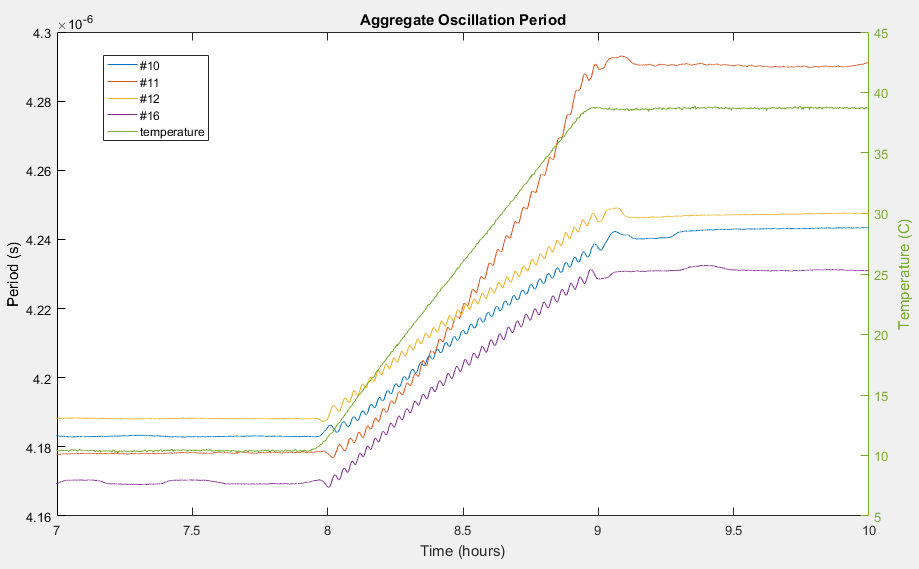
Figure 2. Aggregate oscillation period.
The MAX35103 and MAX35104 can be programmed to return the time of the zero crossings of up to six waves along with time difference measurement, Δτ, or TOF_DIFF. The six waves, called "hit waves" hereafter, can be used to measure the aggregate oscillation period, as follows:
pα = hu(n + 1) + hd(n + 1) - hu(n) - hd(n)
where,
pα = the aggregate oscillation period
n = the particular hit wave time value to use in the calculation. 0 < n < 6 (larger n values are typically better).
hd = the hit wave time value in the down direction
hu = the hit wave time value in the up direction
For example, an application can use hit waves No. 6 and No. 5 to calculate pα, as follows:
pα = hu(6) + hd(6) - hu(5) - hd(5)
The aggregate oscillation period is the sum of the received waveform period as measured by the difference of two adjacent hit values.
Note that the aggregate oscillation period, pα, is twice the period of the average transducer oscillation period as seen by the receiver. Average oscillation period might be a more intuitive measurement, but the constant 2 denominator isn’t mathematically significant once compensation is applied, so aggregate oscillation period is used instead.
Adapting Equation 7 and Equation 8 to use aggregate oscillation period, we get Equation 8 and Equation 9, as follows:
c1 = (Δτ2 - Δτ1)/Pα1 - Pα2)
c2 = (Pα2Δτ1 - Pα1Δτ2)/(Pα1 - Pα2)
where,
Δτ1 = the mean Δτ during stable τ1 temperature
Δτ2 = the mean Δτ during stable τ2 temperature
pα1 = first point aggregate oscillation period
pα2 = tsecond point aggregate oscillation period
Figure 3 shows the final test that was run using the compensation method described in Equation 6 for each device under test. The figure relates compensated (Δτ,right,orange) and uncompensated (Δτ,left,blue) time difference measurements.
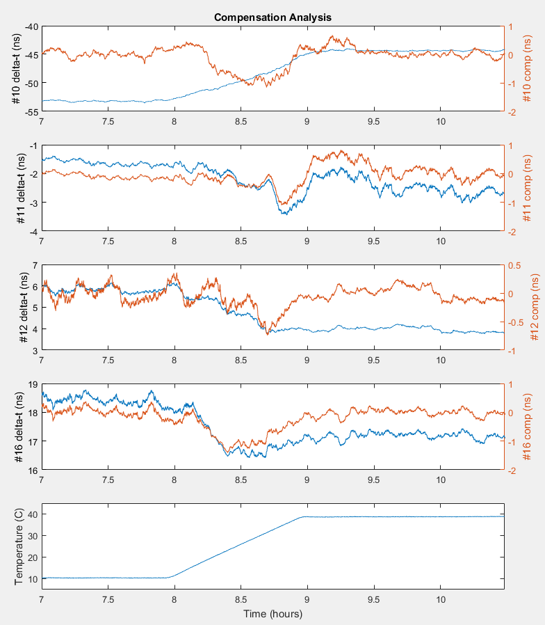
Figure 3. Compensation analysis.
As can be seen, the compensation method presented in this application note reduces transducer-related time errors to within one standard deviation of baseline. The table below provides more detail.
| DUT ID# | Δt1 error | Δ'τ error |
| 10 | -5.16E-08 | -1.30E-10 |
| 11 | -1.81E-09 | -1.05E-10 |
| 12 | 5.45E-09 | -8.71E-12 |
| 16 | 1.81E-08 | -3.03E-11 |
Further Research
Close inspection of the results reveal that increased errors occurs during temperature changes. This hints at the possibility of higher-order terms in the transducer time-error phenomenon. Some applications might require high-order compensation functions such as:
ƒe(τ) = c1t2 + c2t + c3
Constant calculation for this equation is not discussed in this application note. The reader is referred to mathematical sources on polynomial curve fitting. Other types of curve fitting might be applicable, as well. It may also be the case t hat there is a temperature differential contributor to aggregate oscillation period.
Supporting Data
MATLAB® was used to organize and analyze the transducer data. The transducer data set and MATLAB (2016a or later) scripts are available for download at the following address:
EV Kit Software
Alternatively, you can locate the MATLAB package on the MAX35104 product page, under the design resources tab at the following address:
The MATLAB scripts contained in the package contain implementations of the calibration and compensation algorithms presented here.
report.m—This script generates the chart above using cal.m.
dt.m—Extracts delta-t from the given TOF hit value array.
cal.m—Returns a structure containing calibration and compensation information for report.m.
cal_coefs.m—Returns coefficients given delta-t array, aggregate period array, and two-point calibration ranges.
per.m—returns aggregate period array given a TOF hit value array.
comp.m—Returns compensated delta-t given the aggregate period and the calibration coefficients.
quad.mat—contains the raw hit value and temperature data used in the final test.
Conclusion
Differences in paired ultrasonic transducers cause substantial time errors that must be compensated for in software. Temperature and aggregate oscillation period can be used in a two-point linear compensation algorithm to correct for transducer time error.
{{modalTitle}}
{{modalDescription}}
{{dropdownTitle}}
- {{defaultSelectedText}} {{#each projectNames}}
- {{name}} {{/each}} {{#if newProjectText}}
-
 {{newProjectText}}
{{/if}}
{{newProjectText}}
{{/if}}
{{newProjectTitle}}
{{projectNameErrorText}}
最新メディア 21