Considering GSPS ADCs in RF Systems
Abstract
Next-generation radio platforms are moving to a direct RF sampling architecture at an increasing pace. This architecture can significantly reduce the size, weight, and power (SWaP) of the radio, but it introduces the new challenge of needing to simulate the data converter as an RF device, rather than a baseband device. This article will provide a methodology for analyzing GSPS ADCs in RF systems.
Introduction
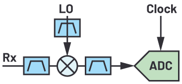
The last 20 years have seen incredible advancements in analog-to-digital converter (ADC) sample rates, from less than 100 MSPS being state-of-the-art in the year 2000, to current data converters often sampling higher than 10 GSPS. As the sample rate of the ADC has increased, so has the input frequency and instantaneous bandwidth that the data converter can digitize. This increasing frequency has allowed for GSPS ADCs to eliminate heterodyning stages, as shown in Table 1, and pull the data converter closer to the RF antenna, enabling a direct RF sampling architecture where no heterodyne stages are required. This transition can cause challenges for system and RF engineers, as the ADC does not behave the same as traditional RF devices such as mixers, amplifiers, and switches. This article is meant to address three critical RF aspects of the GSPS ADC: dynamic range, spurious planning, and noise performance.
| Type | Configuration | Benefits | Challenges |
| Heterodyne |
 |
|
|
| Direct Conversion |
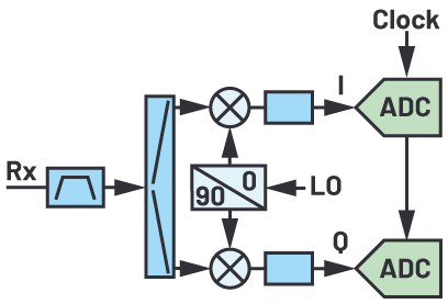 |
|
|
| Direct Sampling |
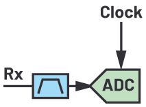 |
|
|
ADC Dynamic Range
Receiver dynamic range is a commonly used performance metric that indicates how small a signal can be and still be received while simultaneously in the presence of very large signals. In a traditional heterodyne receiver, the dynamic range is typically going to be limited by nonlinear RF devices, often a mixer. The two key individual performance metrics that combine to inform dynamic range are noise figure (NF) and input third-order intercept point (IIP3). The NF informs the small signal reception capability, while the IIP3 informs the upper limit on the large signal handling.
Neither NF nor IIP3 are often in the specification table for GSPS ADCs, but the information to extract these parameters is present. First, consider noise figure. In the ADC data sheet these specifications and their associated units are almost always provided (see Table 2).
| Specification | Units |
| Full-Scale (FS) Input Voltage | V p-p |
| Input Impedance (RIN) | Ω |
| Noise Spectral Density (NSD) | dBFS/Hz |
Calculating Noise Figure (NF)
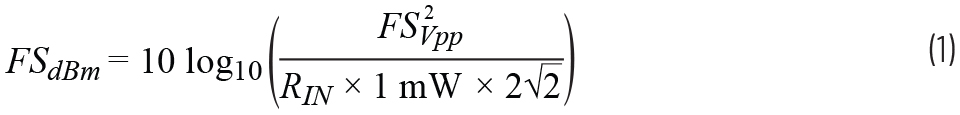
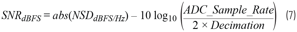
From these three parameters the NF of the GSPS ADC can be calculated. First, the full-scale input voltage needs to be translated from V p-p to dBm.
Second, the noise spectral density (NSD) needs to be converted from a dBFS/Hz parameter into a dBm/Hz parameter.

Finally, the NSD in dBm/Hz is compared against the thermal noise floor to calculate the GSPS ADC NF.

Calculating Input Third-Order Intercept Point (IIP3)
Calculating IIP3 for the GSPS ADC is similarly simple. In the ADC data sheet, the parameters and associated units shown in Table 3 should be present.
| Specification | Units |
| IMD3 Input Power (PIN) | dBFS |
| IMD3 Level | dBc |
To calculate IIP3, the input tones must first be translated to dBm, and then the calculation is straightforward:


Using Equation 4 and 5, the data converter centric parameters specified in the data sheet can be converted into RF parameters for the system and RF design engineer. An example calculation using Equation 4 and 5 is at the end of this article.
Spurious Planning
Another commonly misunderstood concept in GSPS ADCs is the source of, and planning for, significant spurious content. In a traditional heterodyne receiver, the most common source of spurious signals are mixer spurs, specifically M×N mixer spurs. RF and system designs have spur tables, frequency planning, and filter techniques to try to mitigate these mixer spurs. For a direct RF sampling system, there are no M×N spurs because there is no mixer. Instead, the data converter itself is the most significant source of spurs, and so those artifacts must be well understood.
In a heterodyne receiver, the data converter sample rate is set just high enough to satisfy the instantaneous bandwidth required by the receiver channel, typically on the order of 2.5× that bandwidth. In a direct RF receiver, the data converter sample rate could be orders of magnitude higher than what would be required by the instantaneous bandwidth. This is referred to as oversampling, and it has a significant impact on both spurious and noise planning.
The two largest spurious signals of concern in a direct RF sampling architecture are the second harmonic distortion (HD2) and third harmonic distortion (HD3). These spurs can occur within a single Nyquist zone of the ADC, or they could alias, or wrap around, an adjacent Nyquist zone and come back into the desired band. Two examples illustrate this concept. A high speed ADC with a sample rate of 6 GSPS has a first Nyquist zone from DC to 3 GHz, and a second Nyquist zone from 3 GHz to 6 GHz. An input sine wave at a carrier frequency of 800 MHz would create an HD2 product at 1.6 GHz and an HD3 product at 2.4 GHz—in this case, the input tone, HD2, and HD3 are all in the same Nyquist zone. For the second case, increase the carrier frequency from 800 MHz to 1.8 GHz. Now the HD2 product would fall at 3.6 GHz, and the HD3 product would fall at 5.4 GHz—both of which are in the second Nyquist zone. These HD2 and HD3 products will alias to the first Nyquist zone at 2.4 GHz and 600 MHz, respectively. The HD2 product alias in the first Nyquist zone will occur at 2.4 GHz, and the HD3 product alias in the first Nyquist zone will occur at 600 MHz. What is interesting in the second use case is that now the HD2 and HD3 products are both above and below the desired tone. Optimizing this frequency planning is critical for the direct RF sampling architecture and engineer.
A common question is “how much instantaneous bandwidth can I achieve with the highest spurious-free dynamic range (SFDR)?” For a direct RF sampling architecture, this question can be interpreted as “how much instantaneous bandwidth can I achieve while avoiding HD2, HD3, and their alias products?” Analyzing this question is complicated, as the answer will vary with input frequency. There are tools available, such as the Analog Devices Frequency Folding Tool, that can help the engineer understand the potential spurs, but the plot in Figure 1 is a thorough summary for the first and second Nyquist zones.

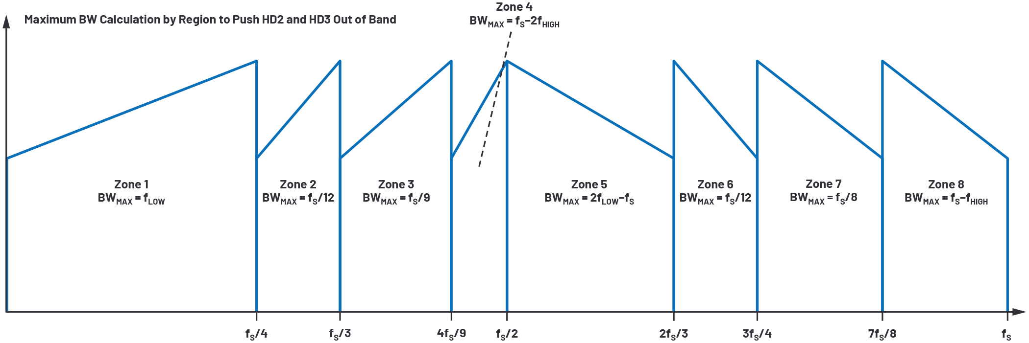
Figure 1. HD2 and HD3 zones for a direct RF sampling ADC.
There are eight zones for bandwidth planning, each with a barrier on a M×divide-by-2 or N×divide-by-3 boundary. In this way, there is similarity to mixer spurious planning. Within a zone, the identified BWMAX is the highest instantaneous bandwidth achievable in that zone—but there will be carrier frequencies and bandwidth combinations that would fall short of that maximum. This chart is meant to give the RF and system engineer an opportunity to optimize sample rate, carrier frequency, and bandwidth decisions in a coherent way that can optimize the receiver’s performance. When a combination of those parameters is selected that avoids HD2 and HD3, then the largest spurs will likely come from clock, power, or isolation effects in the data converter, but those spurious signals are typically 20 dB lower than HD2. This optimization can significantly improve the receiver’s SFDR performance.
Noise Performance
As reviewed, oversampling is important for spurious planning, but it is equally important for noise performance. In a heterodyne receiver, where the ADC sample rate is well matched to the required bandwidth, the noise performance of the data converter directly maps to the noise performance of the receiver. This noise performance is often specified as signal-to-noise ratio (SNR). The other critical noise specification is NSD, as referred to in the section “Calculating Noise Figure (NF).” SNR and NSD are related by:
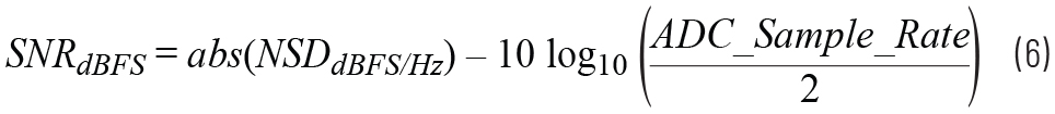
As the NSD performance improves, SNR will also improve. In an oversampled direct RF sampling architecture, the noise in the data converter is not directly mapped to the noise performance of the receiver. The oversampling ratio must also be considered. In an oversampling receiver, the digitized signal must go through decimation filters to realize the desired instantaneous bandwidth. These decimation filters are often half-band or third-band filters, but they could take other orders. As long as the decimation filters themselves are carefully designed, they can provide nearly noise-free bandwidth reduction, which is critical for system noise performance. The overall decimation ratio in a receiver is the cascaded product of all the decimation filter values. For instance, if a receiver used four cascaded half-band filters, then the overall decimation ratio would be 2×2×2×2, or 16. Restating the SNR equation with decimation considered provides the following:
NSD for the ADC is fixed for a given sample rate. Thus, as decimation is increased, the NSD remains constant and the in-band SNR of the receiver will increase. For an ideal decimation filter, this would mean that every decimate-by-2 in the oversampled direct RF sampling architecture would increase SNR by 3 dB. Real-world decimation filters cause some noise degradation, but often it is less than a tenth of a dB per filter. According to the example in Equation 7, a total decimation of 16× will result in an SNR improvement of 12 dB for the receiver—which is very significant!
Putting It All Together
The three concepts mentioned have an interaction that is best understood through an example. The AD9082 is a state-of-the-art, direct RF sampling transceiver with two 6 GSPS ADCs and four 12 GSPS digital-to-analog converters (DACs). For the purpose of this analysis, the focus is only on the ADCs. The performance parameters that are important to the RF and system designer are pulled from the data sheet and listed in Table 4.
| Specification | Value | Units |
| Sample Rate | 6 | GSPS |
| Full-Scale (FS) Input Voltage | 1.475 | V p-p |
| Input Impedance (RIN) | 100 | Ω |
| Noise Spectral Density (NSD) | –153 | dBFS/Hz |
| IMD3 Input Power (PIN) | –7 | dBFS |
| IMD3 Level | –77* | dBc |
| *Data sheet specification is –84 dBFS with a –7 dBFS input, equivalent to –77 dBc | ||
Calculating the important RF parameters covered in this article:
The IIP3 of the AD9082 is greater than 10 dB higher than the NF of the device. This is a critical aspect of dynamic range, indicating that the device is capable of withstanding very large interfering signals while still detecting smaller desired signals. As a point of reference, a high performance mixer often has an NF of ~10 dB and an IIP3 of >20 dBm, also showing a >10 dB gap between the two specifications.
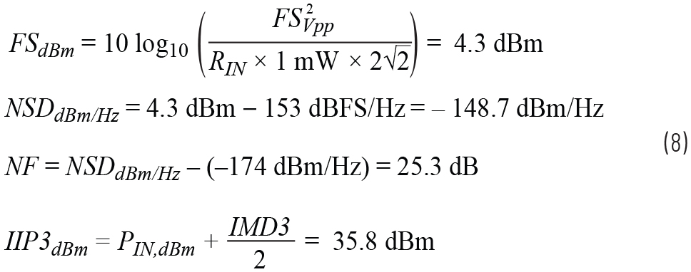
For spurious and noise planning, it makes sense to show the charts together. Figure 2 shows the SFDR and SNR plot for the AD9082 for a 1.2 GHz single-tone input.

Figure 2. Measured SNR and SFDR for the AD9082 vs. decimation.
As the decimation increases, performance improvements for both SFDR and SNR are observed. For SFDR, the increases are obtained by filtering out the HD2 product. As decimation increases from 2× to 4×, the HD2 product falls out of band and is digitally filtered out. For decimation from 8× to 16×, the HD3 product falls out of band and is digitally filtered out. For all decimation settings above 8× the SFDR of the AD9082 is roughly 100 dB or higher. The FFTs of the first and last data point show this increase in performance. Proper frequency planning results in the HD2, HD3, and other spurious products to fall out of band of the desired tone at 1.2 GHz, increasing the SFDR inside of the desired instantaneous bandwidth.

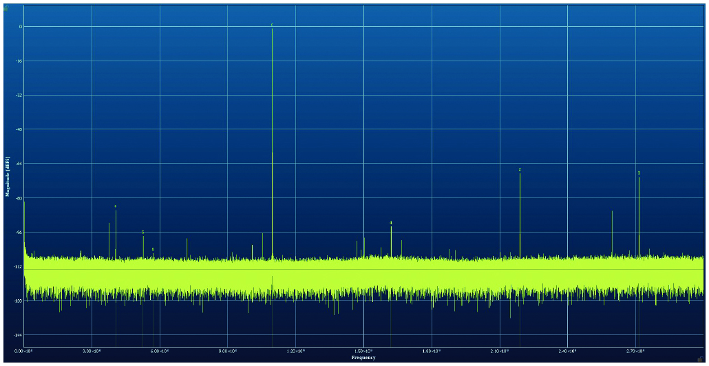
Figure 3. The AD9082 with no decimation. Measured SNR is 56.4 dBFS and measured SFDR is 67 dBc.

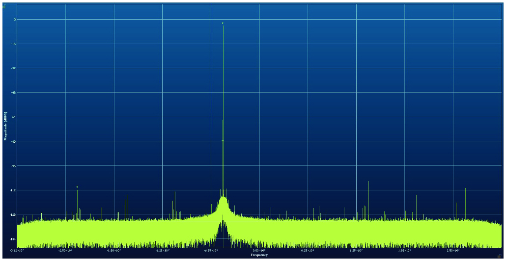
Figure 4. The AD9082 with decimation set to 96×. Measured SNR is 72.8 dB and measured SFDR is 105 dB.
SNR is a more linear improvement, as the decimation filters reduce the amount of integrated noise for the receiver chain. With no decimation, the SNR is 56.4 dBFS; at 8× decimation, the SNR is 63.5 dBFS; and at 96× decimation, the SNR is 72.8 dBFS. As a point of comparison, best-in-class data converter performance for ~100 MSPS devices like the AD9467 and LTC2208 is an SNR of 75 dB and an SFDR of 100 dBc. This class of performance has long been required by the heterodyne signal chains in which ADCs like the AD9467 were commonly used. The AD9082 can achieve the same noise and dynamic range, while eliminating the heterodyne signal chain size, weight, power, and cost—and it is also able to scale to much higher instantaneous bandwidths as required!
Summary
Direct RF sampling architectures provide the RF and system designer with a greater array of design trade-offs than any other architecture. But the flip side of that array is that there are difficult decisions to be made around sample rate, bandwidth, dynamic range, spurs, and noise. Modern direct RF sampling devices, however, are up to the challenge! As shown in the examples in this article, the AD9082 can be programmed to many modalities. In a wideband mode, the AD9082 can achieve SNR of ~56 dBFS and SFDR of ~70 dBc, and through a software reconfiguration to a narrow-band mode the AD9082 can achieve SNR of ~73 dBFS and SFDR of ~105 dBc. That flexibility between narrow-band and wideband modes while maintaining best-in-class performance in both is unique to devices like the AD9082. It also requires that the engineering team designing these direct RF sampling transceivers consider many aspects of receiver design while optimizing the radio design.
About the Authors
Related to this Article
{{modalTitle}}
{{modalDescription}}
{{dropdownTitle}}
- {{defaultSelectedText}} {{#each projectNames}}
- {{name}} {{/each}} {{#if newProjectText}}
-
 {{newProjectText}}
{{/if}}
{{newProjectText}}
{{/if}}
{{newProjectTitle}}
{{projectNameErrorText}}
Latest Media 21