Objective
The objective of this activity is to investigate transformer characteristics in various configurations.
Background
AC Transformer
Transformers only work with alternating current (AC). For example, transformers reduce the 120 V wall power by stepping the voltage down to more convenient levels for most consumer electronics (only a few volts) or for other low power applications (typically 12 V). Transformers also step the voltage up for long distance transmission and down for safe distribution. Without transformers, the waste of electric power in distribution networks, already significant, would be enormous. It is possible to step up or down direct current (DC) voltages, but the techniques are more complicated than with AC transformers and involve turning the DC voltage into some form of AC signal in the process. Further, such conversions are often inefficient and/or expensive. AC has the advantage that it can be used to drive AC motors, which are usually preferable to DC motors for high power applications. While transformers are most visible in power applications, they serve important roles in many other communications related signal paths at audio and RF frequencies.
The transformer core has high magnetic permeability—that is, a material that forms a magnetic field much more easily than in free space due to the orientation of atomic dipoles. In Figure 1, the core is made of laminated soft iron but at higher frequencies ferrite is more common. The result is that the magnetic field is concentrated inside the core, and almost no field lines leave the core.


In certain conditions or scenarios, the magnetic flux ɸ in the primary coil of a transformer is roughly equal to the magnetic flux in the secondary coil. From Faraday’s law, the electromotive force (EMF) in each turn, whether in the primary or secondary coil, is the negative of the derivative of the magnetic flux with respect to time or -dɸ/dt. Neglecting the winding resistance and other losses in the transformer, the terminal voltage equals the EMF. For the Np turns of the primary, this gives:

For the Ns turns of the secondary, this gives:

Dividing these equations gives the transformer equation:

Where r is the turns ratio.
What about the current? Again, neglecting losses in the transformer, and if the voltage and current have similar phase relationships in the primary and secondary, then from conservation of energy we can write in steady state:
Power in = power out,

so:

You never get something for nothing. For a step-up transformer, if you increase the voltage, you decrease the current by (at least) the same factor or turns ratio. Note that, in Figure 1, the coil with more turns has thinner wire, because it is designed to carry less current than that with fewer turns.
Impedance Matching
In communications related applications, transformers are most often used between sections of the circuits to match impedances. As demonstrated, a transformer is capable of converting an AC signal with a certain voltage amplitude at the primary side to a different voltage amplitude at the secondary side. The total power input to the primary and output from the secondary is the same (except for internal losses). The side with the lower voltage is at lower impedance (because this has the lower number of turns), and the side with the higher voltage is at a higher impedance (as it has more turns in its coil).
One example of this impedance matching is a television balun (short for balanced-unbalanced) transformer. This transformer converts a balanced signal from the antenna (via 300 Ω twin lead) into an unbalanced signal (75 Ω coaxial cable such as RG-6). To match the antenna’s 300 Ω source resistance (RS) to the 75 Ω coaxial load resistance (RL), a 4:1 impedance ratio is required. A matching transformer with a 2:1 turns ratio can be used to achieve this. The formula for calculating the transformer turns ratio for this example is:

Frequency Range
The lower limit on the usable frequency range of a transformer is generally set by the impedance level of the circuit in question and the inductance of the transformer windings. If we assume the common 50 Ω standard as our starting point, we can calculate the lower frequency boundary based on the published winding inductance from the manufacturer’s data sheets. The upper limit on the usable frequency range of a transformer is generally set by the parasitic interwinding capacitance and the self-resonance. Typically, data sheets will provide information about the usable frequency range for a component. As a general rule, when selecting the reactive component, such as inductance, it is common practice to choose a value that is at least four times greater than the resistive component, which in this case is the 50 Ω source resistance. This is typically done by considering the lowest frequency of interest.
Formulas Used to Calculate Electrical Characteristics of Multiwinding Transformers
Manufacturer data sheets list certain electrical characteristics for the devices. Probably the most important for our purposes is the winding inductance. For power conversion applications the DC resistance (DCR), the maximum rms current (Irms), and the saturation current (Isat) are also specified.
Connecting Windings in Series:
For higher inductance, multiple windings (WN) can be connected in series. As the inductance increases, energy storage and Irms remain the same, but DCR increases and Isat decreases.

Note: this WN2 factor is only valid when the coupling factor between windings is exactly (or very nearly) one. A more general formula is LT = L1 + L2 + 2M

Where Inductancetable, DCRtable, Isattable, and Irmstable come from the manufacturer’s data sheet.
Connecting Windings in Parallel:
To increase current ratings, multiple windings (WN) can be connected in parallel. DCR decreases, current ratings increase, and inductance remains the same.

Materials
- ADALM2000 Active Learning Module
- Solderless breadboard and jumper wire kit
- One HPH1-1400L 6 winding transformer
- One HPH1-0190L 6 winding transformer
- Two 100 Ω resistors
Directions
Build the circuit shown in Figure 2 on your solderless breadboard. You will be using this setup to measure the frequency response of each of the two transformer model numbers in three different configurations with 1:1 primary to secondary turns ratios. The two red arrows indicate where to connect the source and load resistors for the configuration where one coil is used for the primary and secondary. The blue arrows are for the configuration where two coils in series are used for the primary and secondary. The green arrows are for the configuration where three coils in series are used for the primary and secondary.


Hardware Setup
Open the network analyzer instrument and set the sweep to start at 10 kHz and stop at 10 MHz. The maximum gain should be set to 1×. Set the amplitude to 1 V and the offset to 0 V. Under the Bode scale, set the magnitude top to 10 dB and range to 80 dB. Set the phase top to 180° and range to 360°. Under scope channels, click on use Channel 1 as reference. Set the number of steps to 200.
Procedure
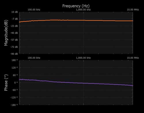
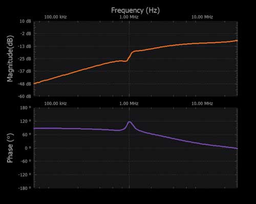
Run a single sweep for each 1:1 winding configuration for the two transformers in your kit of parts. You should see amplitude and phase vs. frequency plots that look very similar to your simulation results. Be sure to export the data to a .csv file for further analysis in either Excel or MATLAB®.

Hardware Setup
Step-Up and Step-Down Configurations
Connect to the transformer for a 1:2 step-up configuration (red arrows) and a 2:1 step-down configuration as shown in Figure 3.


Use the impedance matching formula to calculate the appropriate value for RL in both cases.
Procedure
Repeat the same frequency sweeps using the network analyzer tool. Be sure to export the data to a .csv file for further analysis in either Excel or MATLAB. Compare the measured low frequency roll off points with those measured in the 1:1 configuration from Figure 2.


Question:
- In the context of transformers, what is the purpose of impedance matching and how is it achieved?
You can find the answers at the StudentZone blog.
