Fractional-N PLL with Integrated 6GHz+ VCO Delivers Fractional-N Benefits without Complexity or Performance Downsides
Fractional-N PLL with Integrated 6GHz+ VCO Delivers Fractional-N Benefits without Complexity or Performance Downsides
Jul 1 2014


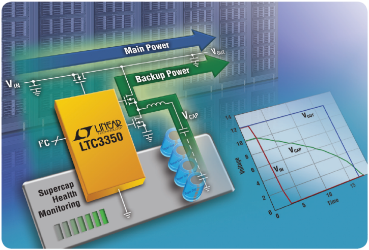
LTC3350 supercapacitor charger and backup controller ensures uninterrupted power in the event of a main power failure.
Fractional-N synthesizers tempt with a number of advantages over integer-N synthesizers, including frequency agility and overall phase noise performance. Even in light of these advantages, PLL system designers rarely yield to the temptation—complex design, poor spurious performance, and delta-sigma modulator noise are generally accepted downsides of using fractional-N synthesizers—but the LTC6948 gives system designers the benefits of fractional-N PLLs without the drawbacks. Unlike typical fractional-N synthesizers, this device is easy to use and yields spurious and noise performance on par with integer-N synthesizers.
The LTC6948 integrates a high end 6GHz-plus VCO in its 4mm × 5mm package, shrinking the size of the PLL system. Furthermore, PLL system design with the LTC6948 is easy with the help of FracNWizard™, a free and sophisticated fractional-N PLL design and simulation tool.
Who Needs a Fractional-N PLL?
The LTC6946 integer-N PLL (LT Journal of Analog Innovation, January 2012) produces a PLL output frequency, fLO(INT_N), that is related to the reference frequency, fREF, as follows:
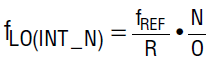
where R is the reference input divide value, N is the VCO feedback divide value, and O is the output divide value.
Figure 1 shows the LTC6946’s simplified block diagram together with the loop filter required to stabilize the loop and an OCXO driving its reference.


Figure 1. Simplified LTC6946 block diagram with external reference clock and loop filter
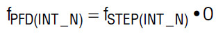
The LTC6946 delivers excellent overall performance, but certain applications require that fLO is moved in small frequency steps, fSTEP(INT_N), or fine-tuned to track a certain frequency with high resolution. Trying to fit an integer-N PLL into such applications would require a very small phase/frequency detector rate, fPFD(INT_N), where
Often, in these situations, fPFD is too small to be practically feasible, but even if it were possible, the in-band phase noise floor, LM(OUT), becomes prohibitively high:
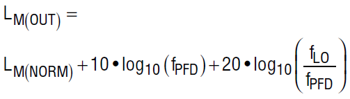
where LM(NORM) is the normalized in-band phase noise floor of the PLL.
Combining the two fPFD terms:
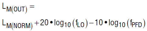
LM(NORM) is fixed for the PLL, so this means that for the same desired fLO, the in-band phase noise floor degrades by −10 • log10(fPFD). In other words, smaller fPFD frequencies make the in-band phase noise floor worse. Figure 2 plots the last equation for an fLO of 6.236GHz while varying fPFD from 10kHz to 100MHz and assuming LM(NORM) = –225dBc/ Hz, the typical normalized constant for the LTC6948 in fractional mode.

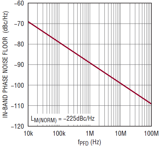
Figure 2. In-band phase noise floor of a PLL at a fixed fLO vs fPFD
Figure 2 shows that fPFD needs to be as high as possible, but it is strongly limited by fSTEP(INT_N), the frequency step size in an integer-N PLL.
Fractional-N PLLs decouple this strong relationship between fSTEP and fPFD. Fractional-N PLLs allow for a much smaller fSTEP than integer-N PLLs while running at a much faster fPFD.
To further investigate the effect of fPFD on the noise contribution of fLO to a communications channel, the phase noise is integrated from 100Hz to 100MHz offset on both sides of fLO = 6.236GHz using practical LTC6948 settings in FracNWizard. Figure 3 summarizes the results.


Figure 3. Double-sideband, 100Hz to 100MHz integrated noise at fLO = 6.236GHz
The integrated noise shown in Figure 3 relates directly to the signal-to-noise ratio (SNR) of the communications channel.
Modern communications channels use complex modulation schemes to maximize data throughput, where an SNR of 40dB or higher is common. Figure 3 shows that a higher fPFD helps meet such requirements.
Under the Hood of the LTC6948
The LTC6948 borrows the high performance phase/frequency detector and VCO from the LTC6946, and adds an 18-bit delta-sigma modulator to the mix to create a world-class fractional-N PLL. Figure 4 shows the block diagram of the LTC6948 along with the loop filter and an OCXO acting as its reference.

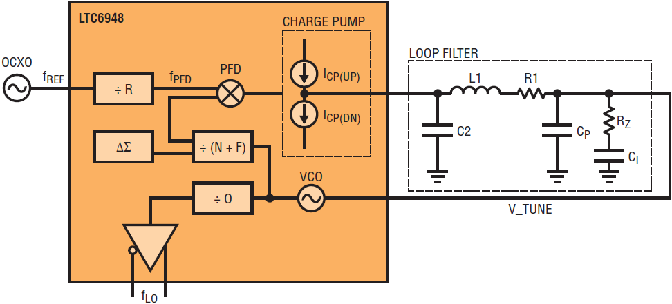
Figure 4. Simplified LTC6948 block diagram with external reference clock and loop filter
For the LTC6948, fLO(FRAC_N) and fREF are related as follows.
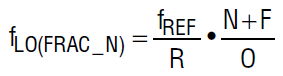
F is the fractional value and is given by
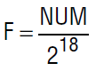
where NUM is the numerator programmed into the delta-sigma modulator internal to the LTC6948. Its value can be any integer between 1 and 218 – 1 (or 262143), meaning 0 < F < 1
As mentioned above, fSTEP(FRAC_N) is small relative to fSTEP(INT_N), despite fPFD(FRAC_N) being typically larger than fPFD(INT_N). This allows the designer to choose the highest possible fPFD(FRAC_N) given fREF, taking advantage of the lowered in band phase noise floor as shown in Figure 2, then verifying that fSTEP(FRAC_N) is small enough to provide the desired frequency resolution at fLO(FRAC_N). The following equation relates the step size to the phase/frequency detector rate.
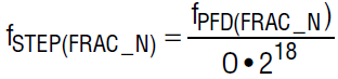
fSTEP(FRAC_N) is 218 times smaller than fSTEP(INT_N) for the same fPFD. For example, an fLO of 6.236GHz can be generated by the LTC6948 with an fPFD of 50MHz resulting in outstanding in-band phase noise floor with a frequency resolution of 190.7Hz (= fSTEP(FRAC_N)). That means the designer can hit any frequency within the VCO range with a maximum error of ±(190.7/2 = 95.4Hz). A maximum error of 95.4Hz out of ~6.236GHz is 0.015ppm (parts per million) or 15ppb (parts per billion), eclipsing the accuracy of virtually any reference clock. Using a larger than one output divide value, O, further shrinks the absolute step size.
Employing a delta-sigma modulator to perform the fractionalization function in a PLL is the preferred method, because a delta-sigma modulator provides high resolution (such as the 218 steps possible with the LTC6948) while intelligently shaping the quantization noise. In other words, the in-band quantization noise is lowered at the expense of higher out-of-band noise. The out-of-band noise is easy to filter out with the help of the passive components shown in Figure 4. As is shown in the “Design Example: Doppler Radar” below, determining the values of these components is straightforward using the FracNWizard software.
The delta-sigma modulator inside the LTC6948 can be shut down, making it run as an integer-N PLL.
Don’t Pay the Usual Price for Fractionalization
Adding a delta-sigma modulator to a PLL can have serious drawbacks, including poor spurious performance (the most significant), delta-sigma modulator noise and design complexity. This is not the case with the LTC6948, as discussed below.
Spurious Performance Overview
A fractional-N PLL has three types of spurious products at its output.
- Reference spurs
- Integer boundary spurs
- Fractionalization spurs
Troublesome spurs are those that are unpredictable. If the location and magnitude of a spur are known, the system designer can either avoid it, or ensure that it does not corrupt the integrity of the system. If the spur’s location and magnitude are random, the designer is left with few good options.
Low Reference Spurs of the LTC6948
Reference (or PFD) spurs are predictable and exist in integer-N PLLs as well. These are located at exactly fPFD and its harmonics away from fLO, centered at fLO. The LTC6948 has excellent reference spur performance. Figure 5 shows the typical performance of the LTC6948 at a ~2.3GHz output.

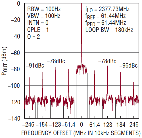
Figure 5. LTC6948 fPFD spurs for fLO = 2.378GHz
Figure 5 shows that with the LTC6948 set to fractional-N mode and generating an fLO of 2.378GHz, the output spectrum contains reference spurs offset from fLO by 61.44MHz (fPFD), and by the harmonics of fPFD. The LTC6948 reference spurs are relatively low in magnitude compared to other devices. Even the most significant spur, 121.88MHz offset from fLO, is inconsequential—it is too low in energy and too far from fLO to cause harm in most real-world applications.
Low and Predictable Integer Boundary Spurs
Integer boundary spurs are physical phenomena inherent to fractional-N PLLs. The VCO output intermodulates with the fPFD harmonics to create beat frequencies. These beat frequencies appear as spurs around fLO only when they are within or near the passband of the loop bandwidth, BW, of the PLL. In other words, when F is extremely close to 0 or 1, these spurs are not attenuated by the loop filter and show up in the spectrum of the PLL output. Figure 6 illustrates this with measurements taken using the LTC6948.


Figure 6. LTC6948 integer boundary spurs for fLO = 2.365GHz (F = 0.00043) to fLO = 2.378GHz (F = 0.4)
As F shifts away from 0 or 1, the integer boundary spurs are attenuated by the loop filter. As F approaches 1/2, 1/3, 1/4, etc., a similar mechanism is in place but at an exponentially lesser extent, so the main integer boundary spurs occur when fPFD • F < BW or fPFD • (1-F) < BW.
In most situations, with careful choice of fREF, and possibly using more than one fPFD and/or fREF, a system designer can avoid these spurs, since their position is known beforehand.
Better yet, and in a good portion of applications, the LTC6948’s integer boundary spur levels (a maximum of –60dBc in the example shown in Figure 6) are so low that they are likely to be below the channel integrated noise in the system. A –40 to –50dBc double-sideband integrated noise in a communications channel is typically considered high end performance, meaning that a maximum of –60dBc spur is still at least 10dB below the channel noise and should not interfere with the overall system performance.
The reduced levels of integer-boundary spurs in the LTC6948, and even unfiltered inside the loop bandwidth, gives it a competitive advantage over other fractional-N PLLs whose integer-boundary spurs often dominate the channel energy.
No Fractionalization Spurs
The LTC6948 does not have unpredictable fractionalization spurs, which infest most other fractional-N devices on the market. The stress of dealing with unpredictable spurs is removed from the LTC6948 equation.
Delta-Sigma Noise
The LTC6948 employs intelligent noise shaping techniques to minimize the in-band noise contribution from the modulator. It boasts a normalized in band phase noise floor, LM(NORM), of –225dBc/Hz in fractional-N mode that compares well with its –226dBc/Hz integer N mode performance. These numbers place the LTC6948 among the PLL elites.
Easy Design
The radar application described below under “Design Example: Doppler Radar” outlines how simple it is to design-in the LTC6948 with FracNWizard software. The LTC6948 does not use a labyrinth of modes, instead using a straightforward design process. All LTC6948 specifications are readily achievable.
VCO Calibration Time
The LTC6948 uses multiple internal VCO sub-bands to cover its entire output frequency range. Each time the LTC6948 is powered up or its frequency is changed, it must be communicated to the IC so it can run an internal search algorithm to apply the correct VCO sub-band.
VCO calibration time should be minimized to limit the PLL lock time. Frequency hopping applications, for example, benefit from fast overall lock times. The LTC6948 can complete its VCO calibration in a little over 10µs as shown in Figure 7. That’s a full order of magnitude faster than most alternative devices.


Figure 7. Typical LTC6948 VCO calibration time
The Often Hidden but All-important 1/F Noise
The reference clock can be the most expensive component in the system. Proper and careful selection of the PLL IC avoids degrading the close-in phase noise, ideally dominated by the reference clock. Often overlooked, the 1/f (or flicker) noise of the PLL IC is an important specification that could degrade the close-in phase noise and negatively affect the in-band phase noise. For instance, Figure 8 shows how the 1/f noise corrupts the in-band phase noise when the 1/f noise corner is elevated. Figure 8 assumes a normalized in-band phase noise floor of –225dBc/Hz.


Figure 8. The effect of different normalized in-band 1/f phase noise specifications on the close-in and in-band phase noise performance
Figure 8 reveals a fact of PLLs that most vendors choose to hide. It shows the strong effect of 1/f noise on the in-band phase noise floor. Even if a PLL IC claims to have an impressive normalized in-band phase noise floor (also known as the figure of merit), it is likely that the same part lacks 1/f noise performance, devaluing the in-band phase noise specification.
The LTC6948 features an impressive –274dBc/Hz normalized in-band 1/f noise specification (normalized with respect to 1Hz offset from an fLO of 1Hz), which is equivalent to a –134dBc/Hz phase noise level for a 100MHz reference clock at an offset of 100Hz, challenging the best 100MHz crystal oscillators available on the market.
The following formula shows how to convert the normalized 1/f number (L1/f) to an offset phase noise value, LOUT(1/f)(fOFFSET), offset by fOFFSET from a certain fLO.

Design Example: Doppler Radar
Doppler radar applications exemplify why 1/f noise performance can be crucial. Doppler radar relies on detecting small frequency shifts inflicted on an incident frequency when reflected by a moving object. The frequency shift, Doppler shift, of a reflected electromagnetic wave, fD, on an incident frequency, fLO, is related to the velocity of the moving object, v, and the speed of light, c, as follows:

Modern uses of Doppler radar include tracking slowly moving objects in surveillance applications. A moderately paced object that is moving at 10mph creates an fD of only 186Hz (assuming c = 671 • 106mph) for an fLO = 6.236GHz. As shown in Figure 8, the 1/f noise performance of the LTC6948 allows the requisite dynamic range at a 186Hz offset, increasing the chances of locating the 10mph moving object. Because the reflected signal is strongly attenuated, sufficient dynamic range in the radar receiver is key to properly deciphering the signal.
Even detection of significantly faster objects benefits from the lower 1/f noise performance of the LTC6948 and its excellent in-band phase noise floor. For instance, a body moving at 200mph has an fD = 3.72kHz if fLO = 6.236GHz.
Figure 8 reveals that a radar system equipped with the LTC6948 allows for the best dynamic range at 3.72kHz offset.
Now that we’ve seen that the performance of the LTC6948 meets the requirements of Doppler radar applications, let’s look at the nuts and bolts of the design process.
Picking the PLL
To design a PLL for the Doppler radar application, where fLO is 6.236GHz, choose the version of the LTC6948 that operates at that frequency. Table 1 shows the four available LTC6948 options.
| VCO Output Divider | Frequency Range (GHz) | |||
| LTC6948-1 | LTC6948-2 | LTC6948-3 | LTC6948-4 | |
| O_DIV = 1 | 2.240 to 3.740 | 3.080 to 4.910 | 3.840 to 5.790 | 4.200 to 6.390 |
| O_DIV = 2 | 1.120 to 1.870 | 1.540 to 2.455 | 1.920 to 2.895 | 2.100 to 3.195 |
| O_DIV = 3 | 0.747 to 1.247 | 1.027 to 1.637 | 1.280 to 1.930 | 1.400 to 2.130 |
| O_DIV = 4 | 0.560 to 0.935 | 0.770 to 1.228 | 0.960 to 1.448 | 1.050 to 1.598 |
| O_DIV = 5 | 0.448 to 0.748 | 0.616 to 0.982 | 0.768 to 1.158 | 0.840 to 1.278 |
| O_DIV = 6 | 0.373 to 0.623 | 0.513 to 0.818 | 0.640 to 0.965 | 0.700 to 1.065 |
The LTC6948-4 includes a VCO that delivers the desired fLO of 6.236GHz.
Designing the PLL
Download FracNWizard at www.analog.com/en/design-center/design-tools-and-calculators and install. The design presented here assumes a 100MHz reference clock—demonstration circuit DC1216A-D from Analog Devices can perform this task. Using FracNWizard (see Figure 9) choose the LTC6948-4, enter the design goals and determine the components required to complete the design.


Figure 9. The FracNWizard tool determines design parameters for fLO = 6.236GHz using the LTC6948
Simulating and Building the PLL
Demonstration circuit DC1959A-D makes a good starting point. Take the filter component values as determined by FracNWizard (sidebar) and replace components on the DC1959A-D as needed with practical value components. Figure 10 shows the schematic of the 6.236GHz circuit with practical filter component values.

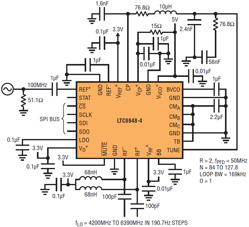
Figure 10. The LTC6948-4 circuit with the calculated loop filter components
Update the FracNWizard filter component values with the practical values of the passive components. As illustrated in Figure 11, FracNWizard predicts the phase noise performance of the LTC6948-4 at the desired 6.236GHz. It shows how the reference phase noise affects the total output noise, helping you choose the reference clock. FracNWizard also shows how the shaped delta-sigma modulator noise is filtered with the use of the passive filter.

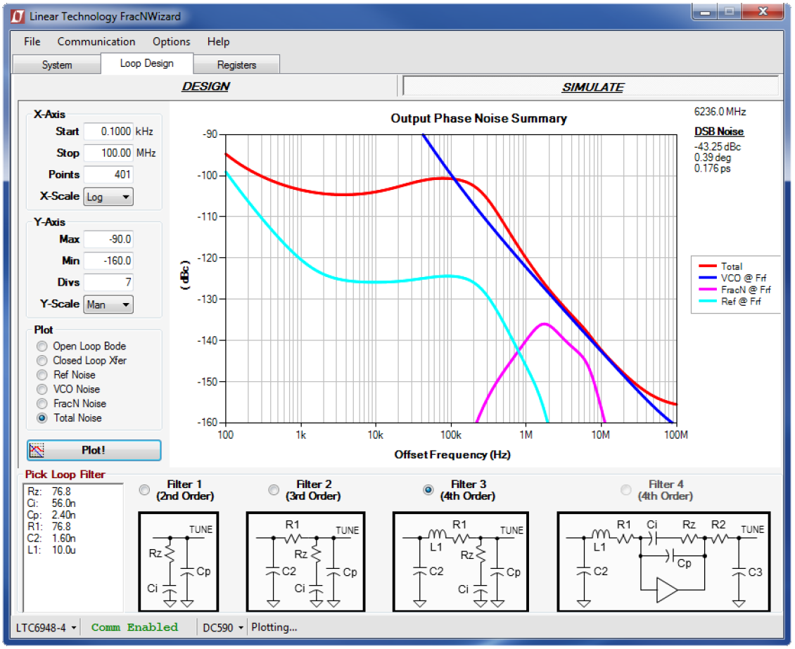
Figure 11. FracNWizard simulation results for fLO = 6.236GHz
Evaluating the PLL
Apply power to the DC1959 and connect it to a PC via demonstration circuit DC590, a USB serial controller available from Analog Devices. Apply the 100MHz reference clock source to the DC1959 and follow the instructions given in the DC1959 demonstration circuit manual at www.analog.com.
Verify the phase noise of our example fLO by connecting the output of the DC1959 to a signal source analyzer, the E5052A from Agilent in this case. Figure 12 shows the result, which aligns closely with the calculated FracNWizard results shown in Figure 11.


Figure 12. Measured results of fLO = 6.236GHz at the output of the LTC6948-4.
That’s it. The fractional-N PLL system design is complete.
Conclusion
The LTC6948 fractional-N PLL offers the benefits of fractionalization, including frequency agility and overall reduced in-band phase noise, without the usual downsides associated with fractional-N PLLs. Design is simplified by free FracNWizard software, and published specifications, although impressive, are conservative and readily attainable.
About the Authors
Michel Azarian is a Senior Applications Engineer at Linear Technology responsible for supporting synthesizer and timing products. Michel holds a bachelor’s degree in Electrical Engineering from the American University of B...
Latest Media 21