"Stitch" Your Way Out of Logic-Analyzer Memory Limitations
Abstract
MATLAB® is a powerful tool that can be used to quickly analyze captured data from an analog-to-digital converter (ADC) output. This application note demonstrates how to use MATLAB to avoid limitations in the memory depth of logic analyzers. Three code-switching methods (basic, advanced, and reverse) are described and compared. Results for all three methods are presented.
Introduction
Characterizing high-speed analog-to-digital converters (ADCs) requires that the digital output codes be captured and analyzed. Limitations in the memory depth of logic analyzers frequently prevent capturing enough data points to create high-resolution FFTs or accurate representations of INL/DNL graphs. A simple way to circumvent this problem is to concatenate multiple sets of data with a mathematical tool such as MATLAB (Figure 1). One drawback of concatenating data is the large discontinuity, which is often present at the point between the two data sets. While the discontinuity makes little difference for INL/DNL graphs, it will wreak havoc on a high-resolution FFT (Figure 2).
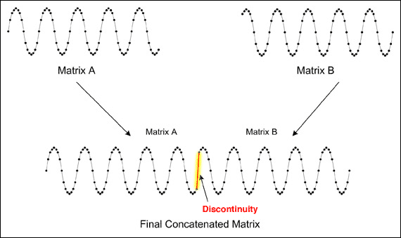
Figure 1. Concatenated data reveals discontinuity between two data sets.
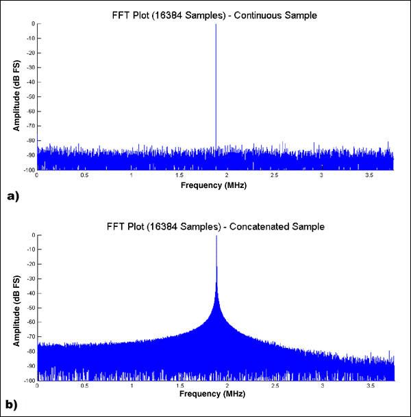
Figure 2. a) A single 16384-point data set was captured and analyzed; b) two 8192-point data sets were captured, concatenated, and analyzed. Stitching Techniques.
One can eliminate discontinuities by searching for identical groups of points (typically three or four) in each data set, and 'stitching' the two data sets together at these points (Figure 3). The easiest way to accomplish this stitching is to record the last four points in the first data set and then search for an identical set of points in the second data set. This position in the second data set is called the 'stitch point.' Any data in the second data set that precedes this stitch point is discarded; the remaining portion of the second data set is attached to the first. This technique is called Basic Code Stitching, is fairly simple to implement, and executes very quickly in MATLAB.
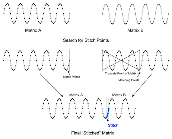
Figure 3. Basic code stitching results in a final "stitched" matrix.
With basic code stitching, sometimes up to half of the second data set needs to be discarded in order to find a set of points that match the last four points of the first data set. Alternatively, discarding a few samples at the tail end of the first data set often helps to find a stitch point closer to the beginning of the second data set (Figure 4). However, looking for a match that discards samples from the tail end of the first data set and the front end of the second data set can be difficult to implement. This process is called Advanced Code Stitching. Finding the ideal stitching point that yields the largest resulting data set requires considerable forethought and programming skill. But if implemented properly, advanced code stitching typically yields a final data set that is at least 90% of the sum of the two smaller data sets.
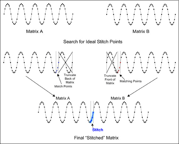
Figure 4. Advanced code stitching looks for ideal stitch points which result in a final "stitched" matrix.
Stitching the second data set (Matrix B) in front of the first data set (Matrix A) is called Reverse Code Stitching and may also result in a larger data set (Figure 5). This technique, however, doubles the processing time because the stitch point must be found when data set A precedes data set B, and when data set A follows data set B. In addition, reverse code stitching typically yields minimal gains when combined with the other stitching techniques. Consequently, due to the substantial increase in processing time required for reverse code stitching, the additional code gains may not be justified on a slower PC. Table 1 details a comparison among the three code-stitching methods.
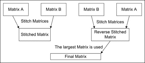
Figure 5. Reverse code stitching doubles processing time, often with minimal code gains.
| Stitch technique | Size of final data set | Description | ||||
| Data set numbers | # of codes (averaged) |
% of two data sets (averaged) |
||||
| 1 + 2 | 3 + 4 | 1 + 4 | ||||
| Concatenate† | N/A | 16384 | 100% | Will produce erroneous FFT; however, INL/DNL can be extracted from this data. | ||
| Basic | 11060 | 8192‡ | 14384 | 11212 | 68.4% | FFT is useable for calculating figures of merit. |
| Reverse | 11060 | 8192‡ | 14384 | 11212 | 68.4% | |
| Advanced | 13790 | 16046 | 16022 | 15286 | 93.3% | |
| Advanced + Reverse |
15427 | 16176 | 16022 | 15875 | 96.9% | |
| *Two 8K (8192 code) data sets were stitched together using the techniques described above. To ensure accuracy, the test was repeated three times using four sets of 8192-point data (labeled 1 through 4). The resultant data from each test was averaged and is presented to the right of the test data. †Concatenation always yields 100% of the available data. ‡Unable to stitch data sets together. |
||||||
MATLAB Functional Description
The attached MATLAB code (StitchMatrices and FindStitchPoint in Appendices A and B, respectively) combines the above topics into one easy-to-use function. These functions accept two data sets (single-column matrices in MATLAB) and several input arguments that enable the advanced-/reverse-code-stitching features. The FindStitchPoint routine identifies offsets in data sets A and B. The StitchMatrices routine discards and combines data sets A and B together using the offsets from the FindStitchPoint routine. In addition, the stitch points in the final data set are recorded in the PrevStitchBins matrix for post-processing. When stitching multiple data sets together, the PrevStitchBins preserves the location of the old stitch points.
Conclusion
Stitching two sets of data together can yield acceptable results. Figure 6 depicts the FFT plot of three 8192-point data sets stitched together (five stitch points used) using the stitching techniques described above. The resulting FFT is almost identical to the 16384-point continuous data set shown in Figure 2a above.
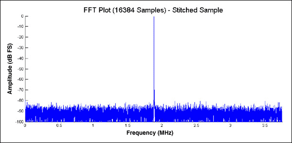
Figure 6. Stitching codes together yields an accurate FFT plot.
Appendix A: StitchMatrices Routine (StitchMatrices.m)
function [StitchedMatrix, StitchBins] = StitchMatrices(MatrixA, ...
                MatrixB, StitchNumber, PrevStitchBins, ...
                AdvCodeStitchEnabled, ReverseStitchEnabled);
%Stitch Matrices Function
%Revision 1.0
%
%By Donald Schelle, May 2005
%Maxim Integrated
%160 Rio Robles
%Sunnyvale, CA, 94086
%
%This function will take two matrices (MatrixA and MatrixB), find a
%given number (StitchNumber) of identical points in each and
%concatenate the two matrices into one.
%
%Inputs = MatrixA, MatrixB (Data Matrices)
%           StitchNumber (Number of points to match)
%            PrevStitchBins (Bins of Previous Stitches in MatrixA)
%            AdvStitchEnabled (0 = NO, 1 = YES)
%            ReverseStitchEnabled (0 = NO, 1 = YES)
%Output = StitchedMatrix (MatrixA + MatrixB)
%            StitchBins (bins of StitchedMatrix where the two
%                           matrices were joined.)
%
%If the matrices can not be joined the function will output a NaN
%for both the StitchedMatrix variable and the StitchBins variable
%--------------------------------------------------------------------------

%Check to see that there are at least TWO StitchNumber Points
if StitchNumber < 2,
   %Requested less than 2 stitch points
   StitchedMatrix = NaN;
   StitchBins = NaN;
   return;
end;

%Calculate Size of MatrixA and MatrixB
[SizeA, Junk] = size(MatrixA);
[SizeB, Junk] = size(MatrixB);

%Find the Stitch Points in MatrixB
[NormalA, NormalB] = FindStitchPoint(MatrixA, MatrixB, ...
                    StitchNumber, AdvCodeStitchEnabled);
%Calculate the size of the NormalStitched Matrix
NormalStitchedSize = NormalA + SizeB - NormalB + 1;

%Check to see if the reverse function is enabled
if ReverseStitchEnabled == 1,
   %Find Stitch Points for Reverse Matrices
   [ReverseB, ReverseA] = FindStitchPoint(MatrixB, MatrixA, ...
                        StitchNumber, AdvCodeStitchEnabled);
   %Calculate the size of the Revered Stitched Matrix
   ReverseStitchedSize = ReverseB + SizeA - ReverseA + 1;
else
   %Set Values to defaults
   ReverseStitchedSize = NaN;       %MatrixB/A Stitch Size
   ReverseA = NaN;
   ReverseB = NaN;
end;

%Check to if it's possible to stitch two matrices
if isnan(NormalStitchedSize) & isnan(ReverseStitchedSize) == 1,
   %The two matrices could not be stitched
   StitchedMatrix = NaN;
   StitchBins = NaN;
   return;
end;

%--------------------- Normal Matrix Stitching Routine ---------------
if (NormalStitchedSize >= ReverseStitchedSize)| ...
            isnan(ReverseStitchedSize) == 1,
   %Stitch MatrixB to the end of MatrixA
   StitchedMatrix = cat(1, MatrixA(1:NormalA), MatrixB(NormalB:SizeB));

   %Update Stitch Bins
   if isnan(PrevStitchBins) == 1,
      %There are no previous stitch bins
      StitchBins = [NormalA, NormalA + StitchNumber - 1];
   else
      %There are previous stitch bins
      %Check for Snipped Stitches
      [SizeStitchBins, Junk] = size(PrevStitchBins);

      while (PrevStitchBins(SizeStitchBins, 2) > (NormalA - 1)),
         %Second Bin is snipped from matrix. Check if first bin is snipped.
         if (PrevStitchBins(SizeStitchBins, 1) > (NormalA - 1)),
            %First Bin is snipped too. Delete Bin Pair
            PrevStitchBins = PrevStitchBins(1:(SizeStitchBins-1),:);
         else
            %First Bin is not snipped but second bin is snipped
            %Shrink Stitch Size
            PrevStitchBins(SizeStitchBins, 2) = NormalA - 1;
         end;

         %Calculate size of new PrevStitchBin Matrix
         [SizeStitchBins, Junk] = size(PrevStitchBins);
      end;

      %Insert New StitchBins
      [SizeStitchBins, Junk] = size(PrevStitchBins);
      StitchBins = PrevStitchBins;
      StitchBins(SizeStitchBins + 1, :) = ...
      [NormalA, NormalA + StitchNumber - 1];

      %Check to see if the last two stitches need to be combined
      [SizeStitchBins, Junk] = size(StitchBins);
      if StitchBins(SizeStitchBins,1) == ...
            (StitchBins((SizeStitchBins - 1),2) + 1),
         %Combine Stitches
         StitchBins((SizeStitchBins - 1),2) = StitchBins((SizeStitchBins),2);
         %Shorten StitchBin Matrix
         StitchBins = StitchBins(1:(SizeStitchBins - 1),:);
      end;

   end;
end;


%--------------------- Reverse Matrix Stitching Routine ---------------
if (ReverseStitchedSize >= NormalStitchedSize)| ...
            isnan(NormalStitchedSize) == 1,
   %Stitch MatrixA to the end of MatrixB
   StitchedMatrix = cat(1,MatrixB(1:ReverseB), MatrixA(ReverseA:SizeA));

   %Update Stitch Bins
   if isnan(PrevStitchBins) == 1,
      %There are no previous stitch bins
      StitchBins = [ReverseB, ReverseB + StitchNumber - 1];
   else
      %There are previous stitch bins
      %Check for Snipped Stitches
      while (PrevStitchBins(1,1) < (ReverseA + StitchNumber - 1)),
         %First Bin is snipped from matrix. Check if second is snipped
         if (PrevStitchBins(1,2) < (ReverseA + StitchNumber - 1)),
            %Second Bin is snipped too. Delete Bad Pair
            [SizeStitchBins, Junk] = size(PrevStitchBins);
             PrevStitchBins = PrevStitchBins(2:SizeStitchBins, :);
         else
            %Second Bin is not snipped, but first bin is snipped
            %Shrink Old Stitch Size
            PrevStitchBins(1,1) = ReverseA + StitchNumber - 1;
         end;
      end;

      %Offset Stitch Bins by inserted amount
      StitchBins = PrevStitchBins + ReverseB - ReverseA + 1;
      %Make Room for new StitchBins
      [SizeStitchBins, Junk] = size(PrevStitchBins);
      StitchBins(2:SizeStitchBins+1, :) = StitchBins;
      %Insert New Stitch Bins
      StitchBins(1,:) = [ReverseB, ReverseB + StitchNumber - 1];

      %Combine close stitches
      if StitchBins(1,2) == StitchBins(2,1) - 1,
         %Combine Stitches
         StitchBins(2,1) = StitchBins(1,1);
         %Shrink Stitch Bins Matrix
     [SizeStitchBins, Junk] = size(StitchBins);
         StitchBins = StitchBins(2:SizeStitchBins,:);
      end;

   end;
end;
Appendix B: FindStitchPoint Routine (FindStitchPoint.m)
function [OutputBinA, OutputBinB]=FindStitchPoint(MatrixA, MatrixB, ...
                MatchNumber, AdvancedStitchFindEnabled)
%Find Stitch Points Function
%Revision 1.0
%
%By Donald Schelle, May 2005
%Maxim Integrated
%160 Rio Robles
%Sunnyvale, CA, 94086
%
%This function will find the IDEAL stitch point in Matrix B given
%the number of data points to match
%
%Inputs = MatrixA
%            MatrixB
%            Number of Records to Match
%            Advanced Stitch Find Enabled (0 = NO, 1 = YES)
%Output = (OutputBinA) End Bin of MatrixA to stitch data
%            (OutputBinB) Start Bin of Matrix B to stitch data
%
%If no bins are found, the function will output a NaN
%--------------------------------------------------------------------------

%Do argument error checking to see if there is enough arguments
if nargin < 2,
   %The user has not supplied enough arguments
   disp('Function requires TWO Matrices');
   OutputBinA = NaN;
   OutputBinB = NaN;
   return;
elseif nargin < 3,
   disp('Select a number of points to match');
   OutputBinA = NaN;
   OutputBinB = NaN;
   return;
elseif nargin == 3,
   %Advanced code stitching is NOT enabled
   OutputBinA = NaN;
   AdvancedStitchFindEnabled=0;
end;

%Ensure that Matrix A and B are single ROW matrices
[row col] = size(MatrixA);
if row > col, MatrixA = MatrixA'; end;
[row col] = size(MatrixB);
if row > col, MatrixB = MatrixB'; end;

%Determine Size of Matrices
[Junk, SizeA] = size(MatrixA);
[Junk, SizeB] = size(MatrixB);

%Initialize OutputBinB to NaN (which means that NO stitch points are found)
OutputBinB = NaN;
%Set initial size of BinA
BinA = SizeA - MatchNumber + 1;
%Initialize BinStop Variable
BinStop = SizeA-100;

%Loop to search through Matrix B numerous times.  This loop is only
%excuted once if Advanced Stitch Find is disabled.  The loop will stop when
%the 'ideal' stitch point is found
while BinA > BinStop,
   %Stuff the Match Numbers into a separate Matrix
    MatchMatrix = MatrixA(BinA:BinA+MatchNumber - 1);

   %Find all bins in MatrixB that match the first number of the Match Matrix
    MatchedBins = find(MatrixB == MatchMatrix(1));

   %Compare the 2nd through nth number of the Match Matrix with the
   %prospective series of numbers in MatrixB

   %Calculate the size of the Matched Bins Matrix
   [Junk, SizeMatchedBins] = size(MatchedBins);

   %The advanced stitch mode optimizes search time by eliminating
   %bad stitch points that would result in the final concatenated
   %matrix being smaller than the last set of stitch points
   if isnan(OutputBinB) == 0,
      %A Stitch Point exists from a previous run.  Elimiate bad stitch points
      %Calculate critical Stitch Point
      MatrixSize = OutputBinA + (SizeB-OutputBinB) + 1;
      CriticalBin = BinA + SizeB - MatrixSize - 1;
      %Find maximum number in the MatchMatrix
      BadBin = find(MatchedBins > CriticalBin);
      %Eliminate Bad Bins (if there are any)
      if isempty(BadBin) == 0,
         MatchedBins = MatchedBins(1:BadBin(1) - 1);
      end;
      %Calculate size of new Matched Bins Matrix
      [Junk, SizeMatchedBins] = size(MatchedBins);
   end;

   %loop to cycle through initial matched bins
   for i=1:SizeMatchedBins,
      %Check to make sure that there isn't a MatrixB overrun
      if (MatchedBins(i) + MatchNumber - 1) > SizeB,
         break;
      end;

      %Assume that next few codes will match and set StitchBinGood = true
      StitchBinGood = 1;
      %Initialize MatchMatrixCounter
      Count = 1;
      %Cycle through MatrixB and compare Numbers with the MatchMatrix
      for j=MatchedBins(i):(MatchedBins(i) + MatchNumber - 1),
         if MatchMatrix(Count)==MatrixB(j),
            %Number is good, continue and check next number
         Count = Count + 1;
     else
            %Number is bad, break loop and try next sequence
            StitchBinGood = 0;
         break;
     end;
      end;

      if StitchBinGood == 1,
         %The optimal (first) stitch has been found
         %Record the End bin of MatrixA
         %Record the Start bin of MatrixB
         OutputBinA = BinA;
         OutputBinB = MatchedBins(i) + 1;
         %Calculate the size of the joined Matrix and a new BinStop#
         BinStop = OutputBinA-OutputBinB+1;
         break;
      end;
   end;

   if AdvancedStitchFindEnabled == 1,
      %Advanced Stitch Find is enabled and we should make a new match
      %matrix and search for these numbers
      BinA = BinA - 1;
   else
      %Advanced Stitch Find is disabled and we should end the loop
      break;
   end;
end;

%Check to see if NO Bins Matched
if isnan(OutputBinB) == 1,
   %NO Bins matched
   OutputBinA = NaN;
end;