A previous article1 examined the relationship of the filter phase to the topology of its implementation. This article will examine the phase shift of the filter transfer function itself. While filters are designed primarily for their amplitude response, the phase response can be important in applications such as time delay simulation, cascaded filter stages, and especially process-control loops.
This article will concentrate on the low-pass and high-pass responses. Future articles in this series will examine the band-pass and notch (band-reject) responses, the all-pass response, and the impulse and step responses of the filter.
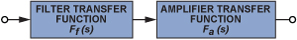
To review, the transfer function of an active filter can be viewed as the cascaded response of the filter transfer function and an amplifier transfer function (Figure 1).
The Low-Pass Transfer Equation
First, we will reexamine the phase response of the transfer equations.
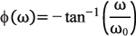
For the single-pole low-pass case, the transfer function has a phase shift given by:
 |
(1) |
where ω represents a radian frequency (ω = 2πf radians per second; 1 Hz = 2π radians per second) and ω0 denotes the radian center frequency of the filter. The center frequency can also be referred to as the cutoff frequency. In terms of phase, the center frequency will be the frequency at which the phase shift is at 50% of its range. Since the radian frequency is used in a ratio, the frequency ratio, f/f0, can be easily substituted for ω/ω0.
Figure 2 (left axis) evaluates Equation 1 from two decades below the center frequency to two decades above the center frequency. Since a single-pole low-pass has a 90° range of phase shift—from 0° to 90°—the center frequency has a phase shift of –45°. At ω = ω0 the normalized center frequency is 1.

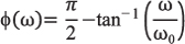
Similarly, the phase response of a single-pole high-pass filter is given by:
 |
(2) |
Figure 2 (right axis) evaluates Equation 2 from two decades below to two decades above the center frequency. The center frequency (=1) has a phase shift of +45°.
If the low-pass pass band is defined as frequencies below the cutoff frequency and the high-pass pass band as frequencies above the center frequency, note that the lowest phase shifts (0° to 45°) are in the pass band. Conversely, the highest phase shifts (45° to 90°) occur in the stop bands (frequencies above low-pass cutoff and below high-pass cutoff).
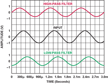
In the low-pass case, the output of the filter lags the input (negative phase shift); in the high-pass case the output leads the input (positive phase shift). Figure 3 shows waveforms: an input sine-wave signal (center trace), the output of a 1-kHz-cutoff single-pole high-pass filter (top trace), and the output of a 1-kHz-cutoff single-pole low-pass filter (bottom trace). The signal frequency is also 1 kHz—the cutoff frequency of both filters. The 45° lead and lag of the waveforms are clearly evident.
For the second order low-pass case, the transfer function’s phase shift can be approximated by:
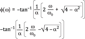 |
(3) |
Figure 4 (left axis) evaluates this equation (using α = √2 = 1.414) from two decades below the center frequency to two decades above the center frequency. Here the center frequency is 1, with a phase shift of –90°.

In Equation 3, α, the damping ratio of the filter, is the inverse of Q (that is, Q = 1/α). It determines the peaking in the amplitude (and transient) response and the sharpness of the phase transition. An α of 1.414 characterizes a 2-pole Butterworth (maximally flat) response.
The phase response of a 2-pole high-pass filter can be approximated by:
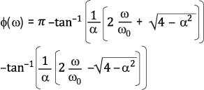 |
(4) |
In Figure 4 (right axis), this equation is evaluated with α = 1.414 from two decades below the center frequency to two decades above the center frequency. At the center frequency (=1), the phase shift is 90°.
Figure 2 and Figure 4 use single curves because the high-pass and the low-pass phase responses are similar, just shifted by 90° and 180° (π/2 and π radians). This is equivalent to a change of the sign of the phase, causing the outputs of the low-pass filter to lag and the high-pass filter to lead.
In practice, a high-pass filter is really a wideband band-pass filter because the amplifier’s response introduces at least a single low-pass pole.
Figure 5 shows the phase- and gain response of a 2-pole low-pass filter, plotted as a function of Q. The transfer function shows that phase change can spread over a fairly wide range of frequencies, and the range of the change varies inversely with the circuit’s Q. While this article is primarily about phase response, the relationship between rate of change of phase and rate of change of amplitude is worth considering.
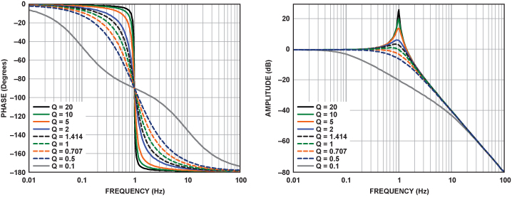
Note that each 2-pole section provides a maximum 180° of phase shift; and at the extremities, a phase shift of –180°, though lagging by 360°, is an angle with the same properties as a phase shift of 180°. For this reason, a multistage filter will often be graphed in a restricted range, say 180° to –180°, to improve the accuracy of reading the graph (see Figures 9 and 11). In such cases, it must be realized that the angle graphed is actually the true angle plus or minus m × 360°. While in such cases there will appear to be a discontinuity at the top and bottom of the graph (as the plot transitions ±180°), the actual phase angle is changing smoothly and monotonically.
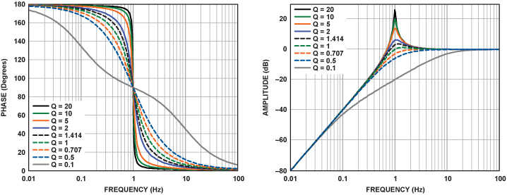
Figure 6 shows the gain- and phase response of a 2-pole high-pass filter with varying Q. The transfer function shows that the 180° of phase change can take place over a large frequency range, and the range of the change is inversely proportional to the Q of the circuit. Also note that the shapes of the curves are very similar. In particular, the phase responses have the same shape, just over a different range.
The Amplifier Transfer Function
The open-loop transfer function of the amplifier is basically that of a single-pole filter. If it is an inverting amplifier, it is in effect inserting 180° of additional phase shift. The closed-loop phase shift of the amplifier is generally ignored, but it can affect the overall transfer of the composite filter if its bandwidth is insufficient. The AD822 was chosen for the simulations of the filters in this article. It affects the composite filter transfer functions, but only at the higher frequencies, because its gain and phase shift are maintained up to considerably higher frequencies than the corner frequency of the filter itself. The open-loop transfer function of the AD822, from the data sheet, is shown in Figure 7.

Example 1: A 1-kHz, 5-pole, 0.5-dB Chebyshev Low-Pass Filter
As an example, we will examine a 1-kHz, 5-pole, 0.5-dB Chebyshev low-pass filter. A few reasons for this specific choice:
1) Unlike the Butterworth case, the center frequencies of the individual
sections are all different. This allows a graph that spreads out the traces
a bit more, so the graph is a little more interesting.
2) The Q’s are generally a bit higher.
3) An odd number of poles emphasizes the difference between single- and
two-pole sections.
The filter sections were designed using the Filter Design Wizard, available on the Analog Devices website.
The f0’s and Q’s of the sections follow:
| f01 = 615.8 Hz | f02 = 960.8 Hz | f03= 342 Hz |
| Q1 = 1.178 | Q2 = 4.545 |
Figure 8 shows the schematic of the complete filter. The filter topology chosen—multiple feedback (MFB)—was again arbitrary, as was the choice to make the single-pole section an active integrator rather than a simple buffered passive RC circuit.

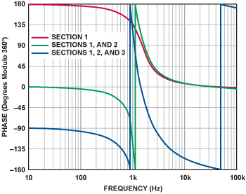
Figure 9 shows phase shifts at each stage of the complete filter. The graph shows the phase shift of the first section alone (Section 1—blue), the first two sections (Sections 1 and 2—red) and the complete filter (Sections 1, 2, and 3—green). These include the basic phase shifts of the filter sections, the 180° contributed by each inverting amplifier, and the effects of amplifier frequency response on overall phase shift.

A few details of interest: First the phase response, being a net lag, accumulates negatively. The first 2-pole section starts with –180° (=180° modulo 360°) due to amplifier phase inversion at low frequencies, increasing to –360° (=0° modulo 360°) at high frequencies. The second section adds another phase inversion starting at –540° (=180° modulo 360°), and the phase increases to –720° (=0° modulo 360°) at high frequencies. The third section starts at –900° (=180° modulo 360°) at low frequencies and increases to –990° (=90° modulo 360°) at high frequencies. Also note that at the frequencies above 10 kHz the phase is rolling off slightly due to the amplifier’s frequency response. That roll-off is seen to be cumulative, increasing for each section.
Example 2: A 1-kHz, 5-pole, 0.5-dB Chebyshev High-Pass Filter
The second example (see Figure 10) considers the phase response of a 1-kHz, 5-pole, 0.5-dB Chebyshev high-pass filter. In this case, the filter was designed (again using the Filter Design Wizard) with Sallen-Key voltage-controlled voltage source (VCVS) sections rather than multiple-feedback (MFB). Though an arbitrary choice, VCVS requires only two capacitors per 2-pole section, rather than MFB’s three capacitors per section, and the first two sections are noninverting.
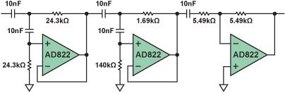
Figure 11 shows the phase response at each section of the filter. The first section’s phase shift starts at 180° at low frequencies, dropping to 0° at high frequencies. The second section, adding 180° at low frequencies, starts at 360° (= 0° modulo 360°) and drops to 0° at high frequencies. The third section, adding a phase inversion, starts at –180° + 90° = 90° at low frequencies, dropping to –540° (= –180° modulo 360°). Note again the additional roll-off at high frequencies owing to amplifier frequency response.
Conclusion
This article considers the phase shift of low-pass and high-pass filters. The previous article in this series examined the phase shift in relation to filter topology. In future articles, we will look at band-pass, notch, and all-pass filters—in the final installment, we will tie it all together and examine how the phase shift affects the transient response of the filter, looking at the group delay, impulse response, and step response.
Appendix
Generic operational equations for single- and two-pole low-pass and high-pass filters are given by equations A1 through A4.
The transfer function of a single-pole low-pass filter:
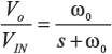 |
(A1) |
where s = jω and ω0 = 2πf0.
The transfer function of a two-pole active low-pass filter:
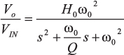 |
(A2) |
where HO is the section gain.
The transfer function of a single-pole high-pass filter:
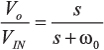 |
(A3) |
The transfer function of a two-pole active high-pass filter:
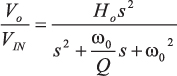 |
(A4) |
The values of f0 and Q for a 1-kHz, 0.5-dB Chebyshev low-pass filter:
| Section | f0 | Q |
| Section 1 | 690.5 | 1.1779 |
| Section 2 | 1017.8 | 4.5451 |
| Section 3 | 362.3 | —— |
For a more detailed discussion, see References 6, 7, and 8.
References
- Zumbahlen, H. “Phase Relations in Active Filters.” Analog Dialogue. Volume 41, No. 4. October 2007.
- Daryanani, G. Principles of Active Network Synthesis and Design. J. Wiley & Sons (1976). ISBN: 0-471-19545-6.
- Graeme, J., G. Tobey and L. Huelsman. Operational Amplifiers—Design and Applications. McGraw-Hill (1971). ISBN: 07-064917-0.
- Van Valkenburg, M.E. Analog Filter Design. Holt, Rinehart & Winston (1982). ISBN: 0-03-059246-1
- Williams, A.B. Electronic Filter Design Handbook. McGraw-Hill (1981).
- Zumbahlen, H. “Analog Filters,” Chapter 5 in Jung, W. Op Amp Applications Handbook. Newnes-Elsevier (2006).
- Zumbahlen, H. Basic Linear Design. Ch. 8. Analog Devices (2006).
- Zumbahlen, H. Linear Circuit Design Handbook. Newnes-Elsevier (2008). ISBN: 978-0-7506-8703-4
